A first network
![]() :
fonsim/examples/a_first_network.md
:
fonsim/examples/a_first_network.md
In this first tutorial a small fluidic network is built and simulated. While still limited in complexity, this simple example shows a typical usage of the FONSim library, including component creation, system definition, simulation and data visualization. In later tutorials, the many aspects of FONSim are explored more in depth.
Note
It might be relevant to note that Python variables are by reference if the variable is mutable. The code example below illustrates this. It prints ‘[4, 2, 3]’ and not ‘[1, 2, 3]’. If it is desired to copy object data and not the reference to it, use the Python copy library.
# Create a List instance.
a = [1, 2, 3]
# Copy the _reference_ to the object.
b = a
# Change variable 'b', which will also change 'a',
# because they point to the same data.
b[0] = 4
# Print 'a' to show that it has been changed.
# This will print '[4, 2, 3]' and not '[1, 2, 3]'.
print(a)
The first step is to import two required modules, Respectively FONSim and Matplotlib. The latter will be used for plotting the simulation results.
# Import fonsim package, for building and simulating a fluidic system
import fonsim as fons
# Import matplotlib package, for plotting the simulation results
%matplotlib inline
import matplotlib.pyplot as plt
Matplotlib is building the font cache; this may take a moment.
Next we create a {py:class:.System} object called ‘system’
to which we will add components.
The ‘system’ object will contain all components in the system
and how these are connected to each other.
# Create a new pneumatic system
system = fons.System()
Here we create and add components to the system.
One of the ways to create a Component instance
is to use FONSim’s standard library,
as is done here with mycomponent = fons.PressureSource....
The object gets label ‘source_00’.
The label can be any string
as long as it only occurs once per system.
The line thereafter,
the created object, named ‘mycomponent’,
is added to the system using the System.add() method.
In the following two lines
the same is done, yet no variable that references to the component,
such as ‘mycomponent’, is kept.
Keeping a variable that references to the component
is not necessary because components can be easily retrieved
by their label
by calling the method System.get()
with as argument the component label
(example: system.get('source_00')).
# Choose a fluid
fluid = fons.air

# Create components and add them to the system
# Note: for now, only take major (pipe friction) losses into account.
mycomponent = fons.PressureSource("source_00", pressure=2e5)
system += mycomponent
system += fons.Container("container_00", fluid=fluid, volume=50e-6)
system += fons.CircularTube("tube_00", fluid=fluid, diameter=2e-3, length=0.60)
The pressure source is instantiated with a constant pressure of 2e5 Pa. Time dependent pressures are also possible, which will be discussed in the next tutorial.
Now that the components are defined, they are connected to each other. Here, no specifics about how exactly the components should be connected to each other are given, and FONSim will therefore choose defaults. After this step, the networked system is fully defined.
# Connect the components to each other.
system.connect("tube_00", "source_00")
system.connect("tube_00", "container_00")
The next step is to simulate the system.
A Simulation instance named ‘sim’ is created
which will hold the system object
and all parameters relevant for the simulation.
Only one simulation parameter is given, namely the duration in seconds
for which the system has to be simulated.
Other parameters, such as the simulation timestep,
are not specified and will therefore be chosen automatically by FONSim.
# Let's simulate the system!
sim = fons.Simulation(system, duration=0.3)
The simulation can now be run:
# Run the simulation
sim.run()
Finally, the simulation results are plotted using the Matplotlib library. For matplotlib tutorials, please refer to the Matplotlib Pyplot introduction.
There are currently two standard ways to plot simulation data.
The first is to manually fetch the simulation data,
plot it and add the legend and axis labels.
The second is to FONSim’s built-in plotting functionality,
which results in quasi the same result as the first option
but with far less work from the user.
This tutorial discusses achieving the same result with both methods.
The first two code lines prepare the plot,
after which the simulation data is plotted.
The simulation data is discretized in the time domain.
The time array is in the Simulation.times attribute
and is accessed here using sim.times.
The simulation data array is accessed through the components.
First, the reference to the component is retrieved from the system,
here using system.get("source_00").
Then, the array is retrieved from the component,
again using ‘get’.
The arguments of the Component.get() method are the label of the variable
and, for some simple components optional, the port.
For example, the tube (CircularTube) has two ports,
which are labeled ‘a’ and ‘b’.
All fluidic components have at least one ‘pressure’ variable
and one ‘massflow’ variable.
A list of the variable and port names of each component type
can be found in the docstring of that component type,
which can be retrieved by calling the help() function on the object
in a Python shell, for example help(system.get("source_00")).
Some IDEs show this docstring after hovering with the mouse
over the code in question.
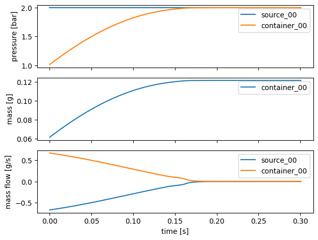
# Manual method
fig, axs = plt.subplots(3, sharex=True, tight_layout=True)
axs[0].plot(sim.times, system.get("source_00").get('pressure')*1e-5, label='source_00')
axs[0].plot(sim.times, system.get("container_00").get('pressure')*1e-5, label='container_00')
axs[0].set_ylabel('pressure [bar]')
axs[1].plot(sim.times, system.get("container_00").get_state('mass')*1e3, label='container_00')
axs[1].set_ylabel('mass [g]')
axs[2].plot(sim.times, system.get("source_00").get('massflow')*1e3, label='source_00')
axs[2].plot(sim.times, system.get("container_00").get('massflow')*1e3, label='container_00')
axs[2].set_ylabel('mass flow [g/s]')
axs[2].set_xlabel('time [s]')
for a in axs: a.legend()
plt.show(block=False)
The simulation arrays denoting a pressure are multiplied with ‘1e-5’ because the simulation results for pressure are stored in unit Pa while the plot y-axis unit is bar (1 bar = 1e5 Pa).
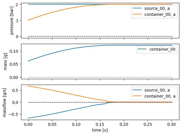
Next, almost the same result is achieved using the FONSim plotting functionality.
The third line
plots the pressure of the components labeled source_00 and container_00
with unit bar.
# Automatic method
fig, axs = plt.subplots(3, sharex=True, tight_layout=True)
fons.plot(axs[0], sim, 'pressure', unit='bar', components=('source_00', 'container_00'))
fons.plot_state(axs[1], sim, 'mass', unit='g', components=('container_00',))
fons.plot(axs[2], sim, 'massflow', unit='g/s', components=('source_00', 'container_00'))
axs[2].set_xlabel('time [s]')
plt.show()
To finish, a brief discussion of the simulation results shown in the figure above. The container pressure in the top graph starts around 1 bar because the simulator assumes that at the start of the simulation there was already some air in the container such that its pressure equalled atmospheric pressure. Therefore the container also starts out with a mass of air of around 0.06 g (middle graph).
As the air flows through the tube from the source to the container, the container fills with air and its pressure increases until its pressure equals that of the source. It is apparent that the system by rough approximation behaves like a first-order linear low-pass filter exposed to a step input.
The bottom plot shows the massflow through the tube (which, the sign not considered, equals that of the source and the container). Of particular interest here are the two flow regimes, turbulent and laminar. Initially, the pressure difference is large, the flow speeds are high, resulting in a high Reynolds number and therefore turbulent flow. Around 0.14 s the massflow has decreased sufficiently for the flow regime to change to laminar, which causes the small ‘bubble’ around 0.16 s.
It is hoped that this first tutorial provided a not-to-steep introduction to FONSim while still providing a good overview of how FONSim is designed to be used.