Balloon actuators

: fonsim/examples/balloon_actuators.md

The previous two examples already showed how to use several main features of FONSim, however, the observed behaviour of the container components was rather simple. Balloon actuators provide a more interesting component and are studied extensively in the field of soft robotics (SoRo). One of their special properties is their nonlinear behaviour. On one hand this makes them somewhat difficult to use for existing applications, but it also opens a wide array of possibilities for new applications such as hardware-encoded sequencing.

Before we dive in, we’ll import a few required packages and get the path to a CSV file that we’ll use later on.

import fonsim as fons
%matplotlib inline
import matplotlib.pyplot as plt
import importlib_resources as ir

# Load example pvcurve CSV file
filepath = 'resources/Measurement_60mm_balloon_actuator_01.csv'
# Use importlib_resources and load as bytestring
# because above file resides in the FONSim package.
# Not necessary for normal files, there one can simply provide the filepath
# as argument for the parameter `data` when initializing the PVCurve object.
ppath = str(ir.files('fonsim').joinpath(filepath))

PV curves

The behaviour of these balloon actuators is specified as a pressure-volume curve or pv-curve. This curve is usually derived from measurements. FONSim contains an example measurements file of a balloon actuator: Measurement_60mm_balloon_actuator_01.csv. This particular example curve was measured as part of the research for this publication.

Let’s have a look at the first five lines of this CSV file:

Latex balloon actuator 60 mm,2017-11-16,MECH1A1
Time,Volume,Pressure
s,ml,mbar
14.31,1,22
17.01,2.01,280

The file is split in four parts (explained more in depth in PVCurve):

• First line: information about the file. For example, the measurement occurred in 2017, November 16.

• Second line: keys of data columns. Here we’re only interested in volume and pressure, though time is listed as well.

• Third line: units of data columns.

• Fourth line and further: the actual numerical data.

Let’s read this file using FONSim and plot the curve. First, the CSV file is loaded into a PVCurve object. The resulting object has two attributes, v and p, which respectively are 1D Numpy arrays of volume and pressures. Their units have been automatically adjusted such they conform to SI base units. The pressure has also been adjusted to absolute because the measured pressure in the CSV file was relative to atmospheric pressure.

# Load pvcurve in PVCurve object
pvcurve = fons.data.PVCurve(data=ppath, pressure_reference='relative')

# Plot the curve
fig, ax = plt.subplots(1, tight_layout=True)
ax.plot(pvcurve.v * 1e6, pvcurve.p * 1e-5)
ax.set_ylabel('absolute pressure [bar]')
ax.set_xlabel('volume [ml]')
plt.show(block=False)
print('Figure 1: PV curve of a balloon actuator')

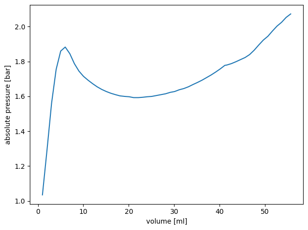
Figure 1: PV curve of a balloon actuator

Figure 1 shows what makes these balloon actuators so interesting: the non-monotonically increasing pressure. As a result, for some pressures there are multiple solutions for the volume of the actuator, three in this case. Note the local pressure maximum of 1.87 bar around a volume of 6 ml (the ‘hill’) and a local pressure minimum of 1.58 bar around a volume of 21 ml (the ‘dip’).

Single balloon actuator

Let’s do a simulation with this balloon actuator! Select a pressure reference and the fluid:

# Pressure reference
waves = [(0, 0.890), (1, 0.650), (2, 0.550), (3, 0.650)]
wave_function = fons.wave.Custom(waves)*1e5 + fons.pressure_atmospheric

# Select a fluid
fluid = fons.air

The previous required a compressible fluid as all components were constant-volume. In this example, the balloon actuators can vary their volume, so feel free to try with an incompressible fluid (for example, water)!

---

Next, the system is built and the simulation is run. The system consists of one pressure source, one balloon actuator (FreeActuator) and a tube connecting the former two.

The FreeActuator component allows to simulate components characterized by a pv-curve and therefore provides an excellent fit for simulating balloon actuators.

# Create system
# The FreeActuator allows to simulate components characterized by a pvcurve.
# The curve argument can take a pvcurve specified as a CSV file.
system = fons.System()
system.add(fons.PressureSource('source', pressure=wave_function))
system.add(fons.FreeActuator('actu', fluid=fluid, curve=ppath))
system.add(fons.CircularTube('tube', fluid=fluid, diameter=2e-3, length=0.60))
system.connect('tube', 'source')
system.connect('tube', 'actu')

# Create and run simulation
sim = fons.Simulation(system, duration=4)
sim.run()

---

Let’s plot the simulation results! Like in the previous example, we’ll use the FONSim built-in plotting functionality:

# Plot simulation results
fig, axs = plt.subplots(3, sharex=True, tight_layout=True)
fons.plot(axs[0], sim, 'pressure', 'bar', ('source', 'actu'))
axs[0].set_ylim(1.4, 2.0)
fons.plot_state(axs[1], sim, 'mass', 'g', ['actu'])
fons.plot(axs[2], sim, 'massflow', 'g/s', ['tube'])
axs[-1].set_xlabel('time [s]')
for a in axs: a.legend()
plt.show(block=False)
print('Figure 2: Simulation output')

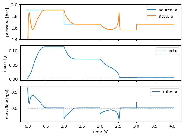
Figure 2: Simulation output

---

To finish, a brief discussion of the simulation results shown in Figure 2. The simulation starts with an increase of absolute pressure to 1.89 bar, the actuator fully inflates as this pressure is larger than the pvcurve hill. Shortly after the pvcurve has been fully inflated, the pressure decreases back to 1.65 bar, just above the pvcurve dip. The actuator therefore stays mostly inflated, as is evidenced by more than half of the mass remaining, shown in the middle graph of Figure 2.

At time = 2.0 s the pressure drops just 0.1 bar, to 1.55 bar. Nevertheless, the actuator now deflates almost fully. Increasing the pressure again at time = 3.0 s has little effect on the actuator volume (middle graph of Figure 2).

Two balloon actuators

In this second simulation, we’ll look at two balloon actuators in series and show a basic example of hardware sequencing achieved by exploiting a combination of actuator nonlinearity and flow restriction. The code is very similar to the previous simulation, so only the relevant differences are discussed here.

Pressure reference, fluid and system:

# Pressure reference
p1 = 0.890
p2 = 0.650
p3 = 0.200
waves = [(0.0, p2),
         (1.0, p1), (1.3, p2),
         (3.0, p1), (3.5, p2),
         (5.0, p3), (5.3, p2),
         (7.0, p3), (7.4, p2)]
wave_function = fons.wave.Custom(waves, time_notation='absolute')*1e5\
                + fons.pressure_atmospheric

# Select a fluid
fluid = fons.air

# Create system
system = fons.System()
system += fons.PressureSource('source', pressure=wave_function)
system += fons.FreeActuator('actu_0', fluid=fluid, curve=ppath)
system += fons.FreeActuator('actu_1', fluid=fluid, curve=ppath)
# Two tubes of respectively 1.20 and 0.60 m
system += fons.CircularTube('tube_0', fluid=fluid, diameter=2e-3, length=1.20)
system += fons.CircularTube('tube_1', fluid=fluid, diameter=2e-3, length=0.60)
# Connect the components together
system.connect('source', 'tube_0')
system.connect('tube_0', 'actu_0')
system.connect('actu_0', 'tube_1')
system.connect('tube_1', 'actu_1')

# Create and run simulation
sim = fons.Simulation(system, duration=9)
sim.run()

# Plot simulation results
fig, axs = plt.subplots(3, sharex=True, tight_layout=True)
fons.plot(axs[0], sim, 'pressure', 'bar', ('source', 'actu_0', 'actu_1'))
axs[0].set_ylim(1.1, 2.0)
fons.plot_state(axs[1], sim, 'mass', 'g', ['actu_0', 'actu_1'])
fons.plot(axs[2], sim, 'massflow', 'g/s', ['tube_0', 'tube_1'])
axs[-1].set_xlabel('time [s]')
for a in axs: a.legend()
plt.show(block=False)
print('Figure 3: Simulation output')

# Also do a parametric plot
rho = fluid.rho if hasattr(fluid, 'rho') else fluid.rho_stp
p_atm = fons.pressure_atmospheric
m_a0 = system.get('actu_0').get_state('mass')
p_a0 = system.get('actu_0').get('pressure')
v_a0 = m_a0 / rho * p_atm / p_a0
m_a1 = system.get('actu_1').get_state('mass')
p_a1 = system.get('actu_1').get('pressure')
v_a1 = m_a1 / rho * p_atm / p_a1

fig, ax = plt.subplots(1, tight_layout=True)
ax.plot(v_a0 * 1e6, v_a1 * 1e6)
ax.set_aspect('equal')
ax.set_xlabel('volume actuator 0 [ml]')
ax.set_ylabel('volume actuator 1 [ml]')
plt.show()
print('Figure 4: Simulation output, actuator volumes')

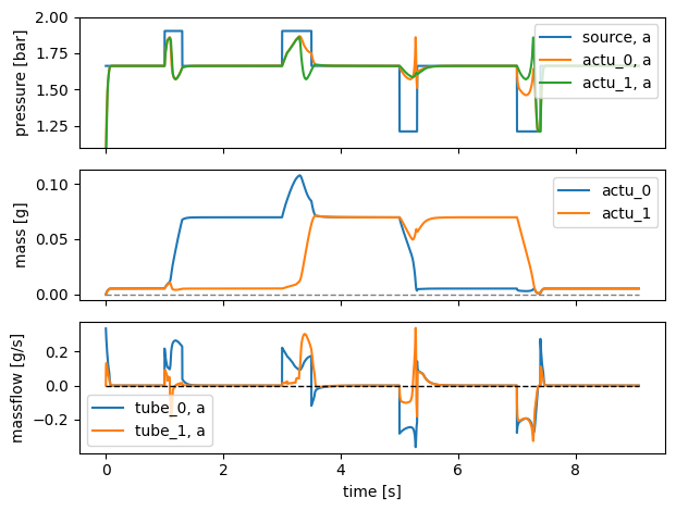
Figure 3: Simulation output

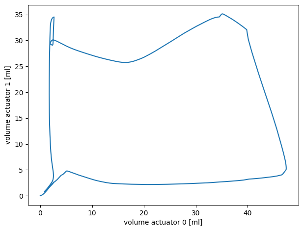
Figure 4: Simulation output, actuator volumes

---

Figures 3 and 4 show the simulation results. The middle graph of Figure 3 shows the achieved phase lag. Even while actuator 0 is inflated first, it is actuator 1 that is deflated last. Also note that the system state between the transitions is stable, as is shown by the constant pressure and mass in these region. These regions can thus be elongated or shortened by changing the pressure reference timings.

This phase lag is also well visible in Figure 4, which plots a virtual path traversed by the actuator volumes. In the research work Hardware Sequencing of Inflatable Nonlinear Actuators for Autonomous Soft Robots, this phase lag was used to produce a stepping motion for a legged robot, where one actuator moved the feet horizontally and another one moved the feet vertically.