A more complex network
![]() :
fonsim/examples/a_more_complex_network.md
:
fonsim/examples/a_more_complex_network.md
This second tutorial extends the network seen in the first with two more tubes and a container. The component connection syntax is elaborated together with the concepts terminal and node. Furthermore, the usage of the built-in wave generator is demonstrated and an introduction to fluids is given.
The following schematic shows the network that will be built and simulated:
            -=- container
   src -=- |
            -=- container
Let’s start by importing FONSim and the plotting package:
import fonsim as fons
%matplotlib inline
import matplotlib.pyplot as plt
In the first tutorial,
the pressure gave a constant pressure.
More useful is if the pressure varies over time.
This is easily achieved using the wave.custom.Custom class
included in FONSim.
Here a simple rectangular wave is chosen.
The desired wave is specified as a list of tuples,
with each tuple of the form (x, y),
with x the time (unit s) where the pressure rises to y (unitless).
In this example, the pressure rises to 0.900 bar relative at t = 0 s,
drops to 0.100 bar relative at t = 0.50 s
and rises to 0.500 bar relative at t = 1.00 s.
The multiplier 1e5 converts the pressures specified in bar
to Pa
and the atmospheric pressure of 1013 hPa (pressure_atmospheric) is added
because FONSim works with absolute pressures
while those specified in the wave are relative.
# Create wave function for pressure source
waves = [(0, 0.900), (0.5, 0.100), (1.0, 0.500)]
wave_function = fons.wave.Custom(waves)*1e5\
                + fons.pressure_atmospheric
The system is constructed,
and the components are defined.
The applicable component equations depend on the used fluid
and therefore it is necessary to specify the fluid
when creating the component.
Given that all components are constant-volume,
a simulation with an incompressible fluid
would be rather boring,
therefore the compressible fluid air is chosen.
FONSim supports Newtonian ideal gasses
with the IdealCompressible class.
Several ideal gasses are included,
see fluids.IdealCompressible.
# Create system
system = fons.System()
# Select fluid
fluid = fons.air
# Create components and add them to the system
system.add(fons.PressureSource('source', pressure=wave_function))
system.add(fons.Container('container_0', fluid=fluid, volume=100e-6))
system.add(fons.Container('container_1', fluid=fluid, volume=100e-6))
system.add(fons.CircularTube('tube_0', fluid=fluid, diameter=2e-3, length=0.10))
system.add(fons.CircularTube('tube_1', fluid=fluid, diameter=2e-3, length=0.02))
system.add(fons.CircularTube('tube_2', fluid=fluid, diameter=2e-3, length=0.70))
Next, connect the components to each other.
Component objects are connected to each other
by assigning their Terminal objects
to a common Node.
Put differently,
terminals that belong to a common node
are considered to be connected to each other,
and the components belonging to these terminals
are also considered to be connected to each other.
In the previous tutorial,
no terminals were specified
and the choice was left to FONSim,
which tends to select a yet unconnected terminal.
Here this behaviour is undesired
as we would like to connect the ends of three tubes
to each other.
The first code line
asks to connect terminal ‘a’ of component ‘tube_0’
to a terminal of component ‘source’.
Terminal ‘b’ of ‘tube_0’
gets connected to terminal ‘a’ of ‘tube_1’ and terminal ‘a’ of ‘tube_2’.
The docstring of the component ought to contain
the labels of the terminals,
see for example CircularTube.
# Connect components to each other
system.connect(('tube_0', 'a'), 'source')
system.connect(('tube_0', 'b'), ('tube_1', 'a'))
system.connect(('tube_0', 'b'), ('tube_2', 'a'))
system.connect('tube_1', 'container_0')
system.connect('tube_2', 'container_1')
Note
The Node objects ought not to be confused
with nodes as they occur in fluidic networks.
FONSim sees a system as a
unidirected graph
with edges/links/lines (FONSim: Component)
and nodes/vertices/points (FONSim: Node).
Sometimes, the FONSim and fluidic meaning of ‘node’
coincide, such as when connecting the ends of three tubes together.
However, most often they do not.
With the system fully defined, the simulation is run. The previous example showed the two manual and automatic plotting methods. The freedom offered by the former is not required here and therefore the latter is used. For plotting the massflow through ‘tube_2’, the terminal to take the massflow from is specified (‘a’) in a similar way as for connecting the components. This gives the plot shown below.
# Create simulation and run it
sim = fons.Simulation(system, duration=1.5)
sim.run()

# Plot results
fig, axs = plt.subplots(3, sharex=True, tight_layout=True)
fig.suptitle("Simulation results")
fons.plot(axs[0], sim, 'pressure', 'bar', ('source', 'container_0', 'container_1'))
fons.plot_state(axs[1], sim, 'mass', 'g', ('container_0', 'container_1'))
fons.plot(axs[2], sim, 'massflow', 'g/s', ('tube_0', 'tube_1', ('tube_2', 'a')))
axs[-1].set_xlabel('time [s]')
plt.show()
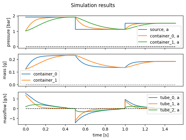
To finish, a brief discussion of the simulation results shown in the figure above. Perhaps first look back on the given tube lengths. The tube from the source to the Y-split has length 10 cm, the tube from the split to the first container (‘container_0’) has length 2 cm and the the tube from the split to the second actuator (‘container_1’) is with 70 cm far longer than the other two tubes.
The pressure (top plot) in the first container behaves similarly to the container in the previously tutorial. It was to be expected that the behaviour of this component is mostly governed by the source as it is much closer to the source than to the other container. Meanwhile, the pressure in the second container shows characteristics of a double first-order low-pass filter, in particular that the pressure curve starts almost horizontally (in an ideal such a filter, it would start perfectly horizontally).
This also shows in massflow through the tubes (bottom plot): the flow through ‘tube_2’ starts from almost zero (even while the source has increased its pressure, little air has yet flown, so both containers maintain their initial pressure).
Feel free to play with the component parameters, such as the diameter and length of the tubes, and see how they influence the simulation results.
The next tutorial will focus on balloon actuators with their pv-curves and nonlinear behaviour.