FONSim introductory example

: fonsim/examples/taste_of_fonsim.md

This example shows a simulation of a pneumatic network popular in soft robotics research that consists of a pressure source and two balloon actuators with identical pvcurves in series, with a restrictor (thin tube) interconnecting the two actuators. The goal of this example is give an impression of what FONSim can be used for. For a more how-to approach, the tutorial A first network is more suitable.

As the simulation results will show, the inflation sequence of the two actuators show a stable phase lag. Such a movement sequence can be used to drive legged robots.

System schematic:

src -=- act -=- act

For a more in-depth discussion and a more gradual introduction to the many features FONSim provides, please refer to this tutorial.

import fonsim as fons
%matplotlib inline
import matplotlib.pyplot as plt
import importlib_resources as ir

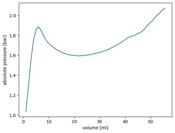
The PV-curve

# Load the PV-curve from a CSV file
filepath = 'resources/Measurement_60mm_balloon_actuator_01.csv'
ppath = str(ir.files('fonsim').joinpath(filepath))
pvcurve = fons.data.PVCurve(ppath)

# Plot the PV-curve
fig, ax = plt.subplots(1)
ax.plot(pvcurve.v * 1e6, pvcurve.p * 1e-5)
ax.set_ylabel('absolute pressure [bar]')
ax.set_xlabel('volume [ml]')
plt.show()

Build the fluidic network

# Pressure reference wave function
p1 = 0.890
p2 = 0.650
p3 = 0.200
waves = [(0.0, p2),
         (1.0, p1), (1.3, p2),
         (3.0, p1), (3.5, p2),
         (5.0, p3), (5.3, p2),
         (7.0, p3), (7.4, p2)]
wave_function = fons.wave.Custom(waves, time_notation='absolute')*1e5\
                + fons.pressure_atmospheric

# Select a fluid
fluid = fons.air

# Create system
system = fons.System()
system += fons.PressureSource('source', pressure=wave_function)
system += fons.FreeActuator('actu_0', fluid=fluid, curve=pvcurve)
system += fons.FreeActuator('actu_1', fluid=fluid, curve=pvcurve)
system += fons.CircularTube('tube_0', fluid=fluid, diameter=2e-3, length=1.20)
system += fons.CircularTube('tube_1', fluid=fluid, diameter=2e-3, length=0.60)
system.connect('source', 'tube_0')
system.connect('tube_0', 'actu_0')
system.connect('actu_0', 'tube_1')
system.connect('tube_1', 'actu_1')

Create and run the simulation

The normal simulation calculation duration on a mid-end laptop is about 6 s. If you’re running this simulation in a Binder instance, the compute resources are limited and you can expect considerably longer durations.

# The simulation duration is set to 9.0 s
# and the timestep is allowed to vary from 1 to 100 ms.
sim = fons.Simulation(system, duration=9.0, step=(1e-3, 1e-1))
sim.run()

Visualize the simulation results

# Time graph
fig, axs = plt.subplots(3, sharex=True, tight_layout=True)
fons.plot(axs[0], sim, 'pressure', 'bar', ('source', 'actu_0', 'actu_1'))
axs[0].set_ylim(1.1, 2.0)
fons.plot_state(axs[1], sim, 'mass', 'g', ['actu_0', 'actu_1'])
fons.plot(axs[2], sim, 'massflow', 'g/s', ['tube_0', 'tube_1'])
axs[2].set_xlabel('time [s]')
for a in axs: a.legend()
plt.show(block=False)

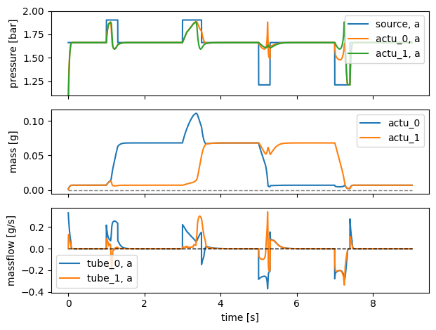
Of particular interest is that in between the pressure source variations (for example, around time 2.0 s, 4.2 s and 6.2 s), the system converges to an equilibrium. This equilibrium can be stretched in time arbitrarily (feel free to try out yourself by playing with the pressure source wave function!). Hence the phase lag is considered to be stable.

# Also do a parametric plot
rho = fluid.rho if hasattr(fluid, 'rho') else fluid.rho_stp
p_atm = fons.pressure_atmospheric
m_a0 = system.get('actu_0').get_state('mass')
p_a0 = system.get('actu_0').get('pressure')
v_a0 = m_a0 / rho * p_atm / p_a0
m_a1 = system.get('actu_1').get_state('mass')
p_a1 = system.get('actu_1').get('pressure')
v_a1 = m_a1 / rho * p_atm / p_a1

fig, ax = plt.subplots(1, tight_layout=True)
ax.plot(v_a0 * 1e6, v_a1 * 1e6)
ax.set_aspect('equal')
ax.set_xlabel('volume actuator 0 [ml]')
ax.set_ylabel('volume actuator 1 [ml]')
plt.show(block=False)

While not visualized explicitly in the figures above, the actuator’s deformation is almost directly related to its volume. Therefore, the defomation is not visualized.